Introduction
Several months ago, when starting this game dev journey, I decided that competent Game AI - that is the intelligence that controls the NPCs - would be an important part of the gameplay experience. And while there are several aspects to getting any solution like that working, whether we are talking behavior trees, HTN (hierarchical task network)1, or GOAP(Goal-Oriented Action Planning)2, the actions the AI characters of the world can take are a key factor. I realized very quickly however, that many actions a character can take involve movement from one location to another. So before I could truly start much of the AI testing, I would need to incorporate some kind of navigation system to move the agents around first.
Research
The Beginning
Naturally, using Unity, my first instinct was to look into using their navmesh solution. The main challenge with this solution was that I required 3D navigation, as some of the AI would be capable of flight. Now I have seen some hacks for this that place a navmesh on walls and other geometry can create links that allow the agents to move between them, but this seemed a little too restrictive to me. The other challenge is that I’m using Unity DOTS and I need a performant experience via jobs. Unity does have an API for this, it is currently marked as Obsolete and could easily be removed in the future.
A second option was the A* Pathfinding Project which, by all accounts, has absolutely glowing reviews. The challenge there was incorporating it with a popular Unity framework I am using called Latios. In the framework I am benefitting from QVVS Transforms and to use the project, I would need to revert to Unity Transforms.
QVVS Transforms provide custom transforms systems based on the concept of QVVS transforms, which are vector-based transforms that can represent non-uniform scale without ever creating shear. This module comes with a fully functional custom transform system with automatic baking and systems, offering more features, performance, and determinism than what is shipped with Unity.
Sparse Voxel Octree - SVO
And thus, I arrived at the conclusion that I would need to implement my own solution. But how to do that? How does one create a 3D navigation system? Well, with a few google searches, it didn’t take me long to find the answer: the sparse voxel octree or as I wil often shorten it moving forward, the SVO. Sparse voxel octrees have uses in ray-tracing, collision detection systems and - what we’re all here for - navigation3. For anyone interested in Game AI in general, GameAIPro has stockpile of articles to keep you busy for quite some time.
Pictures of SVO use cases
Layers
So what’s the difference between the run-of-the-mill octree and an SVO? A normal octree is a data structure where each node subdivides into 8 smaller nodes. The image below shows a great representation where the largest node - the root node - is purple.
Octree Example
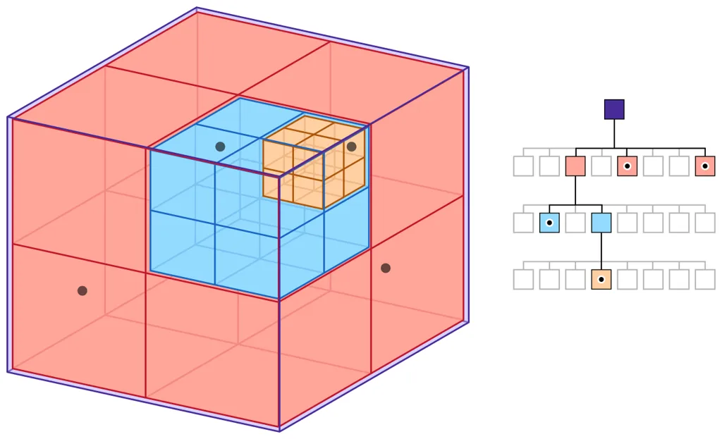
It subdivides into the 8 peach nodes and so on. Thus each subdivision represents a higher resolution of nodes. So an octree 3 layers deep has 1 node at the root layer, 8 at the next layer and 64 at the bottom layer. Each layer here occupies the same amount of space. What changes is the node resolution.
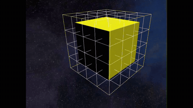
What makes a sparse voxel octree different - well, lots of things make them different -, is that nodes exist only where geometry exists in the world.
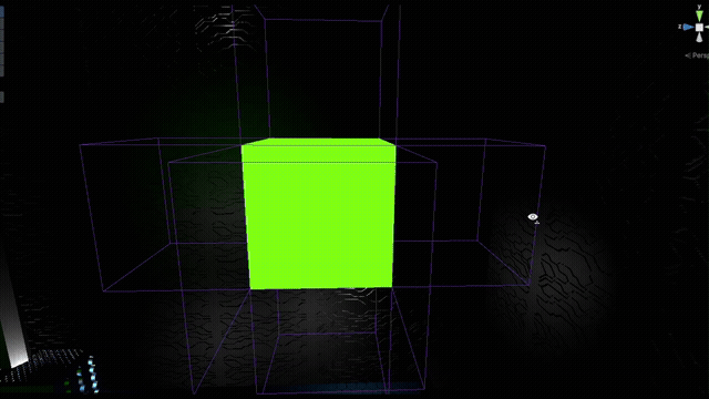
Sparse Voxel Octree Example

In the GIF above I’m showing a simple example a couple of layers deep in an SVO. The top or root layer is not shown explicitly here but it is implied by the 8 node children with the blue outlines. Notice that the next layer down, each of the blue nodes only have 1 child each that contain geometry, corresponding to the location of the cube. Now I highlighted that portion in the last sentence because it is very important to keep in mind. All nodes in an octree with geometry contained within will have 8 children, regardless of whether all 8 children themselves are actually occupied. This is necessary to take advantage of the the fast lookups the octree data structure provides.
Morton Codes / Z-Ordering
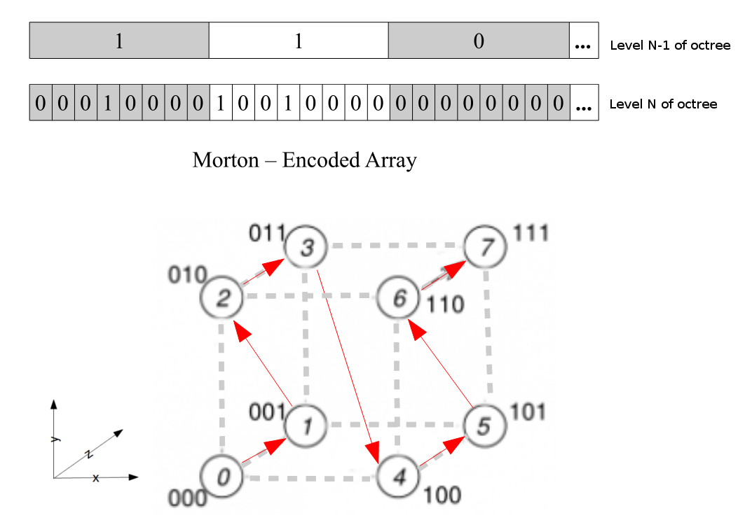
A key feature of an SVO that sets it apart from a traditional octree structure is how the nodes are efficiently stored in memory. Nodes in an SVO are typically stored contiguously in a linear array using Morton codes—also known as Z-ordering. Morton codes are a method for converting multidimensional data, such as three-dimensional node coordinates, into a single-dimensional array. This conversion preserves spatial locality, meaning that nodes close together in 3D space will also be close together in the one-dimensional array.
In the 3D Flight Navigation article3, Figure 21.1c illustrates this beautifully.
Start at the origin point of the diagram and follow the zig-zag progression of the arrows. Notice how the first 7 movements map out the 8 children of a node. Then once we reach the top right corner, the arrow progress to the start of the next node. This means that nodes that are in morton code order, their children will also be stored contiguously in morton code order as well.
Think of each node in a sparse voxel octree as having a 3D grid coordinate that can go from (0, 0, 0) to some max value. Morton encoding take grid coordinate and - using the mysterious power of bitwise operations4 - turns it into an unsigned integer value, ordered based in the zig-zag or z-shaped pattern seen in the image. These morton codes can also be decoded to obtain the grid coordinate.
NOTE: The size of that unsigned value depends on how many layers you want to support in the octree. I’m supporting up to 15 layers(I’ve yet to use more than 8), so there would be a max 8^14 nodes(a lot) on the highest resolution layer, so the unsigned value I am using is a ulong.
If you can’t access that article right now, I suggest also taking a look at the following 2 images:
Shows a higher level node and the grid positions of its 8 children.
At first this may look like a jumbled mess, but wacth the progression of the line carefully, starting in the bottom-left.
For a better, more concise explanation of morton codes, I suggest reading this short article5.
Connectivity
Ok, so we understand that an SVO is sparsely populated and it has nodes that subdivide into smaller nodes, but what makes it so good for navigation? Parent-child links and Neighbors. These two aspects of the structure are what enable connectivity of the 3D space. Before continuing, its important that I mention the SVO - at least in this implementation - is just one long flat array.
Each node has a link to the index of its parent and the index of its first child. Only the first child is necessary because a requirement of the SVO is that a node’s children are stored contiguously. The root node will have its parent marked as -1, but every other node will have a parent index. Similarly, childless nodes use -1 to denote first child index. A node’s neighbors are the 6 nodes adjacent to the node’s 6 faces.
A node in green and its 6 neighbors with purple outlines
You may notice that a node’s neighbors may actually be a node on a different layer. This can happen when the adjacent node of the same layer(same size) does not exist because its parent is childless. Remember, if a node is childless, there is no geometry that exists within its bounds and is therefore empty.
Let’s go ahead and start creating a struct to represent a node
    //  node in an SVO
    public struct Node
    {
        public ulong mortonCode;

        public byte layer;

        // Index of parent node or -1 for root
        public int parentIndex;

        // Always points to 0th octant child(children stored contiguously), -1 for leaf/padding nodes
        public int firstChildIndex;

        // True for padding nodes(childless)
        // Irrelevant for layer 0 nodes(leaf nodes)
        public bool isEmpty;

        // Indices to 6 neighbors (one for each face: +X, -X, +Y, -Y, +Z, -Z)
        // If no neighbor at same level, points to parent's neighbor
        public FixedList32Bytes<int> neighborIndices;
    }
Now we have a slightly better understanding of how nodes link to each other and we can understand if a node is empty - a childless node is empty, whereas one with children means geometry exists somewhere within it. This is fantastic as we make our way down to the bottom layer of the SVO, but once we reach layer 0, AKA the leaf nodes, we have a problem. The nodes give us a coarse representation of obstacles, but we need a fine-grain understanding. Enter voxels stage left.
Note that leaf nodes in a sparse voxel octree are actually the lowest layer (layer 0) or highest resolution nodes, NOT the childless nodes as you may be thinking. Also, it is critical to understand that in this implementation layer 0 contains the leaf nodes and the root node(the highest layer) is at depth - 1. So in a 3-layer SVO, layer 2 contains the root node.
Leaf Nodes & Voxels
I’m sure you’ve heard of these in reference to world of Minecraft or its use for simulating destruction.
Add several images of voxel use cases here - terrain, destruction
I’ve conspicuously left out voxels up until now as their behavior is unique compared to the nodes in the structure. The leaf nodes, as I just mentioned, are at layer 0 and unlike the other layers, it does not contain 8 children but rather maps onto a 4x4x4 voxel grid. To illustrate this, I’ll show the cube example again, but this time I’ll include the voxels with white outline. And lets move it neatly within one leaf node to make it simpler to see.
And now let’s move the cube back to its orginal position.
You can probably see that this give us a much more precise understanding of the geometry and where it exists within the world. Let’s write a quick struct to represent the leaf node and the voxels it contains:
    public struct LeafNode
    {
        // 64-bit array representing 4x4x4 voxel grid
        private BitField64 voxels;
    }
I chose the BitField64 struct because it really fits neatly with our use case. Each leaf node contains 64 voxels to match each bit in the BitField. It already has several useful methods: SetBits(), Clear(), IsSet(), etc. It is also really easy to derive whether the the leaf node is empty => voxels.Value == 0 or if it is fully blocked => voxles.Value == ulong.MaxValue. In fact, let’s update the definition:
    public struct LeafNode
    {
        // 64-bit array representing 4x4x4 voxel grid
        private BitField64 voxels;
        public bool isEmpty => voxels.Value == 0;
        public bool isFullyBlocked => voxels.Value == ulong.MaxValue;
        public bool isOccupied => voxels.Value != 0;
    }
SVO Links
The final piece of the puzzle to round out our understanding of sparse voxel octrees and how they can be used in navigation is the link. Once the SVO has been built, links are used as addresses for different nodes or even voxels within the structure. A link contains layer, node index and subnode index(voxel) information.
“We pack our links into 32 bit integers as follows: 4 bits—layer index 0 to 15 22 bits—node index 0 to 4,194,303 6 bit—subnode index 0 to 63 (only used for indexing voxels inside leaf nodes)”
    /// <summary>
    /// A link/address to a location in the SVO
    /// </summary>
    public struct SVOLink
    {
        private uint packedData;

        public uint Key => packedData;

        // 4 bits - layer index (0-15)
        public byte LayerIndex
        {
            get => (byte)(packedData & 0xF);
            set => packedData = (packedData & ~0xFU) | (value & 0xFU);
        }

        // 22 bits - node index (0-4,194,303)
        public int NodeIndex
        {
            get
            {
                // Check for invalid link (all bits set)
                if (packedData == 0xFFFFFFFF)
                    return -1;

                return (int)((packedData >> 4) & 0x3FFFFF);
            }
            set => packedData = (packedData & ~(0x3FFFFFU << 4)) | (((uint)value & 0x3FFFFFU) << 4);
        }

        // 6 bits - subnode index (0-63) for voxels inside leaf nodes
        public byte SubnodeIndex
        {
            get => (byte)((packedData >> 26) & 0x3F);
            set => packedData = (packedData & ~(0x3FU << 26)) | (((uint)value & 0x3FU) << 26);
        }

        // Create a link from components
        public static SVOLink Create(byte layerIndex, int nodeIndex, byte subnodeIndex = 0)
        {
            SVOLink link = new SVOLink();

            // Handle invalid node index case
            if (nodeIndex < 0)
            {
                // For invalid links, set all bits to indicate invalid state
                link.packedData = 0xFFFFFFFF; // All bits set to indicate invalid
                return link;
            }

            // Pack the data directly without using the properties to avoid double-packing
            link.packedData = ((uint)layerIndex & 0xF) |
                       (((uint)nodeIndex & 0x3FFFFF) << 4) |
                       (((uint)subnodeIndex & 0x3F) << 26);
            return link;
        }

        public static SVOLink CreateFromKey(uint key)
        {
            return new SVOLink { packedData = key };

        }

        // Equal comparison
        public bool Equals(SVOLink other) => packedData == other.packedData;

        // Convert subnode index to 3D coordinates (for leaf nodes)
        public int3 SubnodeToCoords()
        {
            byte idx = SubnodeIndex;
            return new int3(
                idx & 0x3,
                (idx >> 2) & 0x3,
                (idx >> 4) & 0x3
            );
        }

        // Convert 3D coordinates to subnode index (for leaf nodes)
        public static byte CoordsToSubnode(int x, int y, int z)
        {
            return (byte)((z & 0x3) << 4 | (y & 0x3) << 2 | (x & 0x3));
        }
    }
These links make it possible for the pathfinding algorithm to find a clear path through the environment from point a to b. These won’t be too important for a while, as we still need to actually build the SVO first, but I thought I’d go ahead and cover it.
Implementation - Building the SVO
Ok, what we’re all here for. How do we actually transform the theory and concepts into code? As a reminder, I am following this amazing chapter from the GameAIPro3 book, available for free online. I also used an implementation in Unreal Engine - Aeonix Navigation - as inspiration6.
Low Resolution Rasterization
The first step in building our SVO is determining how many leaf nodes we’ll actually need. This might seem backwards - why not just start with the finest detail and work our way up? The answer lies in efficiency and memory allocation. We need to know upfront how much memory to allocate for our entire structure, and the only way to do that is to understand where geometry exists in our world.
The Resolution Hierarchy
Remember from our earlier discussion that if our final voxel resolution is 2 meters, then our leaf nodes (layer 0) will be 4×2 = 8 meter cubes. But here’s a crucial insight from the GameAIPro3 chapter: the parent of a leaf node will always have to be split. This is because if we have geometry that requires leaf node detail, we need at least two leaf nodes next to each other in each direction to provide meaningful navigation options.
This means we can perform our initial rasterization at layer 1 (16 meter resolution) instead of layer 0. We’re essentially asking: “Which 16-meter cubes in our world contain geometry?” For each one that does, we know we’ll need to create 8 leaf nodes beneath it.
The Rasterization Process
Rather than creating a full 3D grid (which would be memory-intensive), we use a clever approach: we maintain a sorted list of unique Morton codes representing the occupied nodes. This gives us all the spatial information we need while keeping memory usage minimal.
// Get all obstacle colliders and their transforms
*obstacleColliders = *obstacleQuery.ToComponentDataArray<Collider>(Allocator.Persistent);
*obstacleTransforms = *obstacleQuery.ToComponentDataArray<WorldTransform>(Allocator.Persistent);

// Rasterize at layer 1 resolution
var lowResJob = new LowResRasterizationJob
{
    Colliders = _obstacleColliders,
    Transforms = _obstacleTransforms,
    Settings = svoSettings,
    MortonEncoder = _mortonEncoder,
    LayerOneNodeSize = svoSettings.GetNodeSize(1), // 16m for our example
    MortonCodes = _mortonCodesHashSet.AsParallelWriter(),
}.Schedule(_obstacleColliders.Length, 64, state.Dependency);
The LowResRasterizationJob does the heavy lifting here. For each collider in our scene, it:
- Calculates the AABB (Axis-Aligned Bounding Box) of the collider in world space
- Transforms to grid space relative to our octree’s origin
- Determines which grid cells the AABB overlaps
- Generates Morton codes for each overlapped cell
Let’s break down the job implementation:
[BurstCompile]
private struct LowResRasterizationJob : IJobParallelFor
{
    // ... fields ...

    public void Execute(int index)
    {
        var collider = Colliders[index];
        var transform = Transforms[index];

        // Calculate the AABB for this collider
        var aabb = Physics.AabbFrom(collider, transform.worldTransform);

        // Transform to grid space (relative to octree origin)
        float3 gridSpaceMin = (aabb.min - (Settings.origin - Settings.extents)) / LayerOneNodeSize;
        float3 gridSpaceMax = (aabb.max - (Settings.origin - Settings.extents)) / LayerOneNodeSize;
The grid space transformation is critical here. We’re converting from world coordinates to our octree’s coordinate system. The expression (Settings.origin - Settings.extents) gives us the bottom-left-back corner of our octree’s bounds - our grid’s origin point.
Grid Coordinate Conversion
Next, we convert our floating-point grid coordinates to integer grid indices:
// Convert to integer grid coordinates (floor for min, ceil for max to ensure coverage)
int3 gridMin = new int3(
    (int)math.floor(gridSpaceMin.x),
    (int)math.floor(gridSpaceMin.y),
    (int)math.floor(gridSpaceMin.z)
);
int3 gridMax = new int3(
    (int)math.floor(gridSpaceMax.x),
    (int)math.floor(gridSpaceMax.y),
    (int)math.floor(gridSpaceMax.z)
);
You might wonder why I’m using floor for both min and max instead of floor for min and ceil for max. This is because we’re dealing with grid cell indices, not continuous space. A collider that extends from grid position 1.1 to 1.9 only occupies grid cell 1. Using ceil for max could cause us to mark empty grid cells as occupied.
We then clamp these coordinates to ensure they stay within our octree’s bounds:
// Clamp to valid grid bounds
int gridRes = Settings.GetGridRes(1);
gridMin = math.max(gridMin, new int3(0, 0, 0));
gridMax = math.min(gridMax, new int3(gridRes - 1, gridRes - 1, gridRes - 1));
Morton Code Generation
Finally, we iterate through all overlapped grid cells and generate their Morton codes:
// Generate Morton codes for all overlapped voxels
for (int x = gridMin.x; x <= gridMax.x; x++)
{
    for (int y = gridMin.y; y <= gridMax.y; y++)
    {
        for (int z = gridMin.z; z <= gridMax.z; z++)
        {
            MortonCode mortonCode = Morton.EncodeMorton3D_LUT(new uint3((uint)x, (uint)y, (uint)z), ref MortonEncoder);
            MortonCodes.Add(mortonCode);
        }
    }
}
The NativeParallelHashSet automatically handles duplicate Morton codes for us. If multiple colliders occupy the same grid cell, we’ll only store that cell’s Morton code once.
Converting to Sorted List
After the rasterization job completes, we convert our hash set to a sorted list:
var initializeCodesJob = new InitCodesJob
{
    MortonCodeHashSet = _mortonCodesHashSet,
    LowResCodes = _lowResOccupiedCodes,
}.Schedule(lowResJob);
This sorting step is crucial because it ensures our Morton codes are in spatial order, which will be important for the subsequent steps in our SVO construction.
Generating Leaf Nodes
Now comes the payoff. For each layer 1 Morton code, we generate 8 leaf nodes:
var genLayer0Nodes = new GenerateLayerZeroOctreeNodes
{
    LayerOneMortonCodes = _lowResOccupiedCodes,
    MortonDecoder = _mortonDecoder,
    MortonEncoder = _mortonEncoder,
    OctreeNodes = _octreeNodes.AsParallelWriter()
}.Schedule(_lowResOccupiedCodes.Length, 64, state.Dependency);
The GenerateLayerZeroOctreeNodes job uses bit manipulation to efficiently generate child Morton codes:
public void Execute(int index)
{
    MortonCode layerOneMorton = LayerOneMortonCodes[index];

    // Generate 8 children directly using bit operations
    for (uint childIndex = 0; childIndex < 8; childIndex++)
    {
        ulong childMorton = (layerOneMorton << 3) | childIndex;
        // ... create node ...
    }
}
This bit manipulation is elegant: we shift the parent’s Morton code left by 3 bits (making room for the child index) and then OR in the child index (0-7). This gives us the Morton codes for all 8 children in the correct spatial order.
Memory Allocation Success
After sorting our layer 0 nodes, we know exactly how much memory our SVO will require. We can allocate one contiguous block and initialize our first layer:
// Sort Layer 0 Nodes
_octreeNodes.Sort();
// Initialize octree layer 0
var layer0 = _octreeLayers[0];
layer0.LayerIndex = 0;
layer0.NodeStartIndex = 0;
layer0.NodeCount = leafNodeCount;
layer0.NodeSize = svoSettings.leafSize;
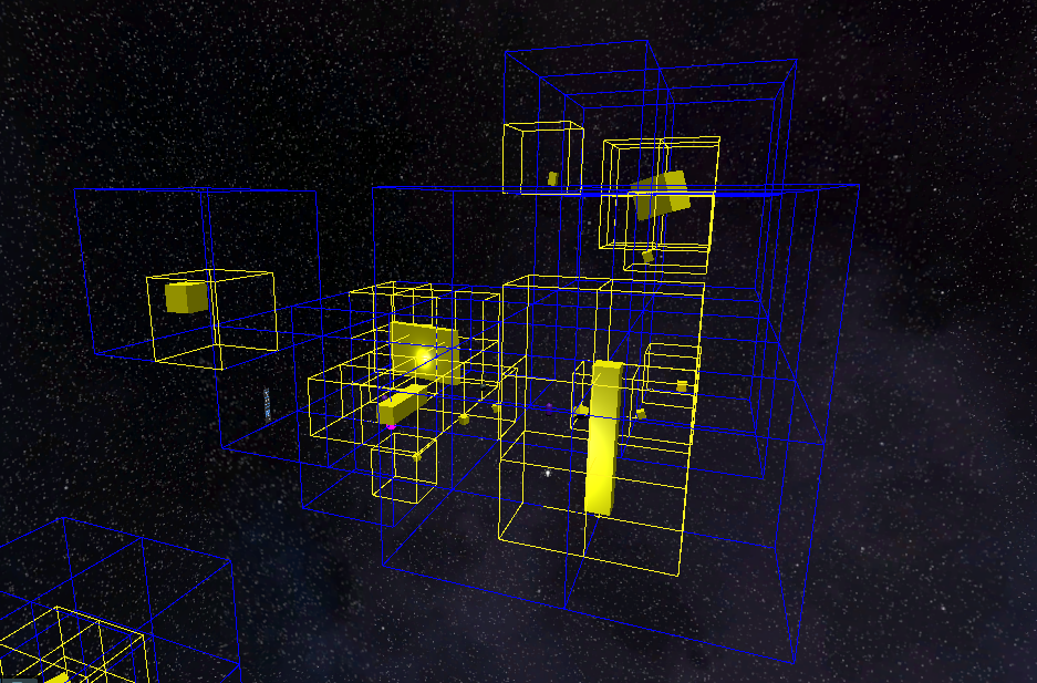
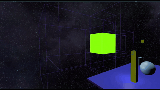
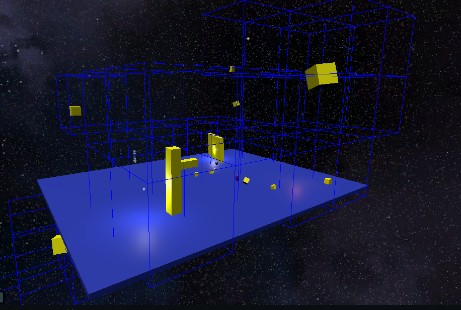
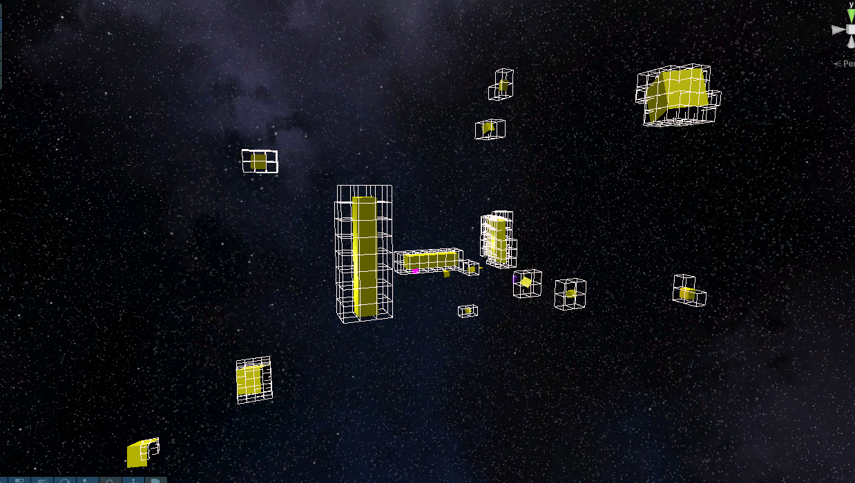
_octreeLayers[0] = layer0;Low Res Rasterization - Column - NOTE: Only the yellow objects in the scene are considered obstacles.
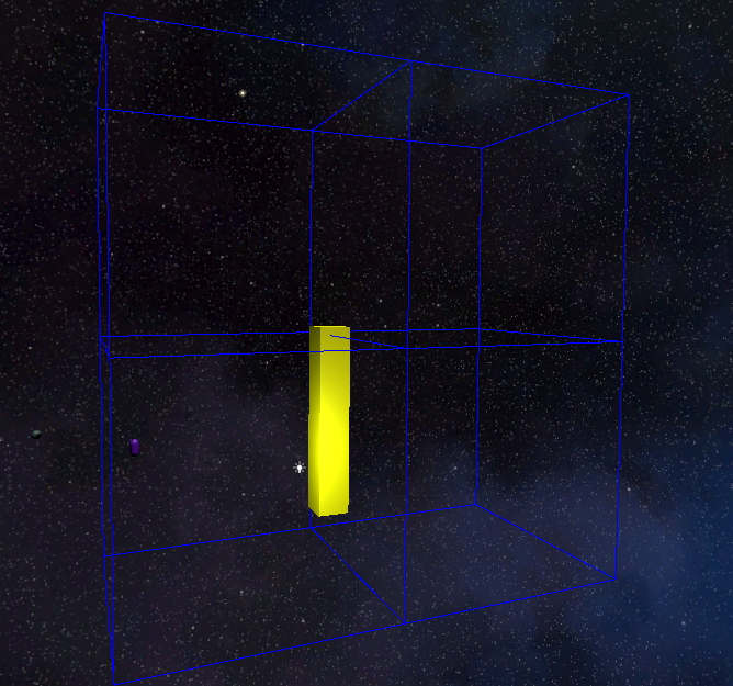
Low Res Rasterization - Full Scene
At this point, we have successfully completed the low-resolution rasterization phase. We know where all our leaf nodes will be positioned and have allocated the memory for them. The next step will be to work our way up the tree, creating parent nodes and establishing the hierarchical relationships that make the SVO so powerful for navigation.
The beauty of this approach is its efficiency - we’ve avoided creating unnecessary nodes in empty space while ensuring we have adequate detail wherever geometry exists. This sparse representation is what makes SVOs so effective for 3D navigation in complex environments.
Bottom-Up Layer Construction
Now that we have our leaf nodes (layer 0) properly positioned, we need to build the rest of our octree structure. This is where the “bottom-up” approach comes into play - we start with our detailed leaf nodes and progressively create parent nodes up to the root. This process establishes the hierarchical relationships that make our SVO navigable and maintains the spatial organization that makes queries efficient.
The Parent-Child Relationship Challenge
Here’s where things get interesting, and potentially confusing. In a traditional octree, nodes only exist where needed. But for our SVO to be efficient during pathfinding, we need a crucial guarantee: every non-leaf node must have exactly 8 children. This might seem wasteful, but it’s what allows us to perform fast octant-based traversals during navigation queries.
The problem is that our initial leaf nodes are sparse - they only exist where geometry is present. So when we create parent nodes, some of those 8 child slots will be empty. Rather than leaving gaps, we create “padding nodes” - placeholder nodes that represent empty space but maintain our octree’s structural integrity.
Building Layer by Layer
Let’s walk through the construction process layer by layer:
// Bottom-up construction - create padding nodes for missing children
for (int currentLayer = 0; currentLayer < svoSettings.maxDepth - 1; currentLayer++)
{
int nextLayer = currentLayer + 1;
var currentLayerInfo = _octreeLayers[currentLayer];
// Extract unique parent Morton codes from current layer
var parentMortonCodes = new NativeParallelHashSet<MortonCode>(
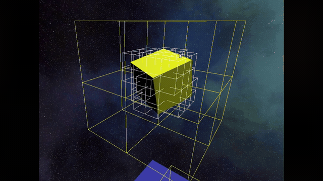
svoSettings.GetMaxNodesInLayer(nextLayer), Allocator.TempJob);Layer 0 & 1 - Column
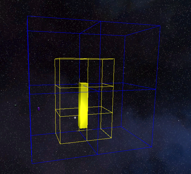
Layer 0 & 1 - Cube
Layer 0 & 1
For each layer, we start by identifying which parent nodes we need to create. This is where the beauty of Morton codes shines - we can derive a parent’s Morton code directly from any child’s code using bitwise operations.
Extracting Parent Morton Codes
The ExtractParentMortonCodesJob does exactly what its name suggests:
[BurstCompile]
struct ExtractParentMortonCodesJob : IJobParallelFor
{
    [ReadOnly] public NativeArray<OctreeNode> ChildNodes;
    [WriteOnly] public NativeParallelHashSet<ulong>.ParallelWriter ParentMortonCodes;

    public void Execute(int index)
    {
        var childNode = ChildNodes[index];
        ulong parentMorton = Morton.GetParentCode(childNode.mortonCode);
        ParentMortonCodes.Add(parentMorton);
    }
}
The GetParentCode method:
public static MortonCode GetParentCode(MortonCode child)
{
    return child >> 3;
}
Remember our earlier discussion about Morton codes and the Z-ordering pattern? The last 3 bits of a Morton code represent which of the 8 octants (children) a node occupies within its parent. By shifting right by 3 bits, we’re effectively removing the octant information and getting the parent’s Morton code. It’s that simple, and it’s incredibly fast.
The parallel hash set automatically deduplicates parent Morton codes for us. Multiple children can share the same parent, but we only want to create each parent node once.
Creating Padding Nodes
Here’s where our implementation gets more complex than the basic algorithm description. After we have our unique parent Morton codes, we need to ensure that every parent will have exactly 8 children:
// Create padding nodes for missing children
// Layer 0 already padded in STEP ONE (job that generates layer 0 nodes)

int addedPadding = 0;
if (currentLayer > 0)
{
    for (int parentIdx = 0; parentIdx < parentNodeCount; parentIdx++)
    {
        MortonCode parentMortonCode = sortedParentCodes[parentIdx];

        // Create all 8 children for this parent
        for (uint childOffset = 0; childOffset < 8; childOffset++)
        {
            MortonCode childMortonCode = Morton.GetChildCode(parentMortonCode, childOffset);

            // Look for existing child in current layer
            int existingChildIndex = FindNodeByMortonCode(currentLayerInfo, childMortonCode);

            if (existingChildIndex == -1)
            {
                // Create padding node
                OctreeNode childNode = new OctreeNode
                {
                    layer = (byte)currentLayer,
                    mortonCode = childMortonCode,
                    parentIndex = -1,
                    firstChildIndex = -1,
                    neighborIndices = new FixedList32Bytes<int>(),
                    isEmpty = true
                };
                _octreeNodes.Add(childNode);
                addedPadding++;
            }
        }
    }

    // Sort all nodes to maintain Morton code ordering
    _octreeNodes.Sort();
}
Notice that we skip layer 0 for padding creation. Why? Because we already created a complete set of 8 leaf nodes for each layer 1 Morton code during our low-resolution rasterization step. Layer 0 is already “padded” with the full set of children.
For subsequent layers, we use the inverse operation to GetParentCode:
public static MortonCode GetChildCode(MortonCode parent, uint childOctant)
{
    return (parent << 3) | childOctant;
}
We shift the parent’s Morton code left by 3 bits (making room for the octant) and then OR in the child’s octant index (0-7). This generates the Morton codes for all 8 potential children.
The Binary Search Helper
To check if a child already exists, we use a binary search:
private int FindNodeByMortonCode(OctreeLayer layerInfo, MortonCode targetMortonCode)
{
    // Binary search since nodes are sorted by morton code
    int left = layerInfo.NodeStartIndex;
    int right = layerInfo.NodeStartIndex + layerInfo.NodeCount - 1;

    while (left <= right)
    {
        int mid = (left + right) / 2;
        MortonCode midMorton = _octreeNodes[mid].mortonCode;

        if (midMorton == targetMortonCode)
            return mid;
        else if (midMorton < targetMortonCode)
            left = mid + 1;
        else
            right = mid - 1;
    }
    return -1; // Not found
}
This works because we maintain our nodes in Morton code order, and Morton codes preserve spatial locality. The binary search gives us O(log n) lookup performance, which is much faster than a linear search when dealing with thousands of nodes.
Creating Parent Nodes
After padding is complete, we create the actual parent nodes. This is where we establish the crucial parent-child links that will enable efficient traversal during pathfinding:
// Find the first child (0th octant) in the sorted array
MortonCode firstChildMorton = Morton.GetChildCode(parentMortonCode, 0);
int firstChildIndex = FindNodeByMortonCode(
    new OctreeLayer
    {
        NodeStartIndex = updatedCurrentLayerInfo.NodeStartIndex,
        NodeCount = updatedCurrentLayerInfo.NodeCount
    },
    firstChildMorton
);

// Create parent node
var parentNode = new OctreeNode
{
    layer = (byte)nextLayer,
    mortonCode = parentMortonCode,
    parentIndex = -1, // Will be set in next iteration
    firstChildIndex = firstChildIndex,
    neighborIndices = new FixedList32Bytes<int>(),
    isEmpty = false
};
The key insight here is that we only store the firstChildIndex in each parent node. Since children are stored contiguously in Morton code order, we can always find child N by accessing firstChildIndex + N. This saves memory and simplifies traversal logic.
The Root Node Special Case
The root node requires special handling because it has no parent and represents the entire octree bounds:
// Special case: maxDepth - 2 layer (children of root)
if (currentLayer == svoSettings.maxDepth - 2)
{
    var rootNode = new OctreeNode
    {
        layer = (byte)(svoSettings.maxDepth - 1), // Root is at maxDepth - 1
        mortonCode = 0,
        parentIndex = -1, // Root has no parent
        firstChildIndex = updatedCurrentLayerInfo.NodeStartIndex, // Points to first child at maxDepth - 2
        neighborIndices = new FixedList32Bytes<int> { -1, -1, -1, -1, -1, -1},  // Root has no neighbors
        isEmpty = false
    };

    _octreeNodes.Add(rootNode);
    // ... update children to point to root as parent ...
}
The root node’s Morton code is always 0, and it has no neighbors (hence all neighbor indices are -1).
Parent Index Prediction
One of the trickier aspects of this bottom-up construction is setting the parentIndex correctly. Since we’re adding padding nodes and sorting after each layer, the indices of parent nodes will change. We need to predict where each parent will end up after the next iteration’s sorting:
// Calculate where this parent will be after next iteration's padding/sorting
MortonCode grandparentMortonCode = Morton.GetParentCode(parentMortonCode);
int parentOctant = (int)(parentMortonCode & 0x7);

int predictedParentIndex;
if (grandparentMortonCode == currentGrandparent)
{
    // Same grandparent - just add the octant offset
    predictedParentIndex = currentGrandparentStartIndex + parentOctant;
}
else
{
    // New grandparent - account for remaining slots of previous grandparent
    currentGrandparentStartIndex += 8; // Move to next grandparent's children
    currentGrandparent = grandparentMortonCode;
    predictedParentIndex = currentGrandparentStartIndex + parentOctant;
}
This prediction works because we know that after padding and sorting, each parent (grandparent) will have exactly 8 children stored contiguously in Morton code order.
The Result
After this process completes, we have a fully constructed octree with several important properties:
- Every non-leaf node has exactly 8 children (including padding nodes for empty space)
- All nodes are stored in Morton code order, enabling efficient spatial queries
- Parent-child relationships are properly established through index references
- Memory is allocated efficiently in a single contiguous block
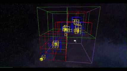
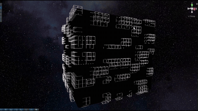
Full SVO Post Bottom-Up Construction
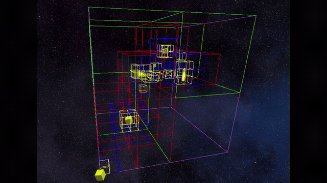
Full SVO Fly Through
This structure is now ready for the next step: establishing neighbor relationships, which will complete our navigation mesh and enable pathfinding algorithms to traverse between adjacent nodes in 3D space.
The bottom-up construction process might seem complex, but it’s this careful attention to structure that makes our SVO incredibly efficient during runtime navigation queries. The time invested in building a well-organized octree pays dividends every time an AI agent needs to find a path through our 3D world.
Set Neighbor Links
With our octree structure complete, we now need to establish the connections that will make navigation possible. This is where neighbor links come into play - the critical relationships that allow pathfinding algorithms to move seamlessly between adjacent nodes in 3D space. Unlike the bottom-up construction we just completed, neighbor link establishment works from the top of the octree down to the leaves.
Why Neighbors Matter
Each node in our SVO needs to know about its 6 face neighbors - the nodes adjacent to its +X, -X, +Y, -Y, +Z, and -Z faces. These links are what transform our octree from a static spatial data structure into a navigable mesh. When a pathfinding algorithm reaches the boundary of a node, it needs to know where it can go next. Neighbor links provide these navigation options.
The Top-Down Approach
The GameAIPro3 chapter describes a key insight: if a node has no neighbor at the same level, then the neighbor link is set to that node’s higher level parent’s neighbor. This hierarchical fallback ensures that every node always has a path to adjacent space, even when the neighboring region has lower detail.
Let’s walk through this process:
/* STEP 3 - Build Neighbor Links
 *
 * Neighbor links are filled in traversing back down the octree. Each node has 6 neighbors, one for each face.
 * If a node has no neighbor for a face at the same level, then the neighbor link is
 * set to that node's higher level parent's neighbor. This ensures that each node always has a link to a
 * neighbor through each of its faces. If a face is on the edge of the octree, then the value is -1.
 *
 * We put faces in this order: +X, -X, +Y, -Y, +Z, -Z
 */

// Skip top layer - root node's neighbors were set during bottom-up construction
for (int layer = svoSettings.maxDepth - 2; layer >= 0; layer--)
{
    var layerInfo = _octreeLayers[layer];
    int limit = layerInfo.NodeCount + layerInfo.NodeStartIndex;

    for (int nodeIndex = layerInfo.NodeStartIndex; nodeIndex < limit; nodeIndex++)
    {
        var node = _octreeNodes[nodeIndex];
        var neighborIndices = new FixedList32Bytes<int>();

        // Convert Morton code to 3D coordinates for this layer
        int3 nodeCoords = (int3)Morton.DecodeMorton3D_LUT(node.mortonCode, ref _mortonDecoder);
        int layerSize = svoSettings.GetGridRes(layer);

        // Check each of the 6 faces
        for (int faceIndex = 0; faceIndex < 6; faceIndex++)
        {
            // ... neighbor finding logic ...
        }
    }
}
Notice that we skip the root layer (maxDepth - 1) because the root node has no neighbors - it represents the entire octree bounds. Its neighbor indices were already set to -1 during the bottom-up construction phase.
Face Direction Mapping
We establish a consistent convention for face directions:
private int3 GetFaceDirection(int faceIndex)
{
    switch (faceIndex)
    {
        case 0: return new int3(1, 0, 0);   // +X
        case 1: return new int3(-1, 0, 0);  // -X
        case 2: return new int3(0, 1, 0);   // +Y
        case 3: return new int3(0, -1, 0);  // -Y
        case 4: return new int3(0, 0, 1);   // +Z
        case 5: return new int3(0, 0, -1);  // -Z
        default: return new int3(0, 0, 0);
    }
}
This ordering is important - it needs to remain consistent throughout our entire system. Pathfinding algorithms will rely on knowing that face index 0 always means the +X direction.
Finding Direct Neighbors
For each face, we first attempt to find a direct neighbor at the same layer:
for (int faceIndex = 0; faceIndex < 6; faceIndex++)
{
    int3 neighborCoords = nodeCoords + GetFaceDirection(faceIndex);

    // Check if neighbor is outside octree bounds
    if (neighborCoords.x < 0 || neighborCoords.x >= layerSize ||
        neighborCoords.y < 0 || neighborCoords.y >= layerSize ||
        neighborCoords.z < 0 || neighborCoords.z >= layerSize)
    {
        neighborIndices.Add(-1); // Outside octree boundary
        continue;
    }

    MortonCode neighborMortonCode = Morton.EncodeMorton3D_LUT((uint3)neighborCoords, ref _mortonEncoder);

    // Search for neighbor at current layer
    int neighborIndex = FindNodeByMortonCode(layerInfo, neighborMortonCode);
    if (neighborIndex != -1)
    {
        // Direct neighbor found at same layer
        neighborIndices.Add(neighborIndex);
    }
    else
    {
        // No direct neighbor - do hierarchical search through parents
        int hierarchicalNeighbor = FindHierarchicalNeighbor(nodeIndex, faceIndex);
        neighborIndices.Add(hierarchicalNeighbor);
    }
}
The process is straightforward:
- Calculate neighbor coordinates by adding the face direction to our current node’s coordinates
- Check bounds - if the neighbor would be outside the octree, mark it as -1
- Convert to Morton code and search for a node at the same layer
- If found, use that as our direct neighbor
- If not found, fall back to hierarchical neighbor search
The Grid Resolution Connection
Notice how we use svoSettings.GetGridRes(layer) to determine the bounds checking:
public int GetGridRes(int layerIndex)
{
    return baseGridRes >> layerIndex;
}
This method calculates the grid resolution at each layer by bit-shifting our base resolution. If our leaf layer (layer 0) has a resolution of 256x256x256, then layer 1 has 128x128x128, layer 2 has 64x64x64, and so on. This halving of resolution at each layer up is fundamental to how octrees work.
Hierarchical Neighbor Search
When we can’t find a direct neighbor at the same layer, we need to search up the hierarchy. This is where the “hierarchical fallback” concept becomes crucial:
private int FindHierarchicalNeighbor(int nodeIndex, int faceIndex)
{
    var currentNode = _octreeNodes[nodeIndex];
    int currentParentIndex = currentNode.parentIndex;

    // Traverse up the hierarchy until we find a parent with a neighbor in this direction
    while (currentParentIndex != -1)
    {
        var parentNode = _octreeNodes[currentParentIndex];

        int parentNeighborIndex = parentNode.neighborIndices[faceIndex];
        if (parentNeighborIndex != -1)
        {
            // Parent has a neighbor - this becomes our hierarchical neighbor
            return parentNeighborIndex;
        }

        // Move up to next parent level
        currentParentIndex = parentNode.parentIndex;
    }

    // Reached root without finding neighbor - must be at octree boundary
    return -1;
}
This function implements a key insight from the GameAIPro chapter: if our current node doesn’t have a direct neighbor, we can inherit the neighbor relationship from our parent. This makes sense spatially - if there’s no node adjacent to us at our level of detail, then we’re at the boundary between regions of different detail levels.
Let’s think through an example. Imagine we have a small obstacle surrounded by open space. The area around the obstacle will have high detail (many small leaf nodes), while the open space has low detail (fewer, larger nodes). A leaf node at the edge of the high-detail region won’t have a direct neighbor leaf node on the open space side. Instead, it will inherit its parent’s neighbor relationship, which points to the larger node representing the open space.
Why Top-Down Works
The top-down approach works because we’re inheriting neighbor relationships from nodes that have already been processed. Since we start at the highest levels (which have the sparsest, most general relationships) and work down to the most detailed levels, each node can safely inherit from its parent.
This also ensures that every node has a path to adjacent space. Even if that path goes through a node at a different level of detail, the pathfinding algorithm can still traverse from one region to another.
Boundary Conditions
Nodes at the edge of the octree deserve special attention. These nodes genuinely have no neighbors in certain directions - they’re at the world boundary. We handle this by setting their neighbor index to -1:
if (neighborCoords.x < 0 || neighborCoords.x >= layerSize ||
    neighborCoords.y < 0 || neighborCoords.y >= layerSize ||
    neighborCoords.z < 0 || neighborCoords.z >= layerSize)
{
    neighborIndices.Add(-1); // Outside octree boundary
    continue;
}
During pathfinding, a neighbor index of -1 signals that movement in that direction would take the agent outside the navigable world space.
The Final Result
After this process completes, every node in our SVO has a complete set of 6 neighbor links. These links either point to:
- Direct neighbors at the same level of detail
- Hierarchical neighbors inherited from parent nodes
- Boundary markers (-1) indicating world edges
Another Neighbor Example
This neighbor network transforms our octree into a true 3D navigation mesh. Pathfinding algorithms can now traverse from any node to any adjacent node, even when those nodes exist at different levels of detail. The hierarchical fallback ensures that transitions between high-detail and low-detail regions are seamless.
With both the octree structure and neighbor relationships established, our SVO is nearly ready for navigation. The final step will be the leaf rasterization, where we populate the finest level of detail with actual voxel data representing the precise location of obstacles within each leaf node.
Leaf Rasterization
We’ve reached the final and most detailed step of our SVO construction: leaf rasterization. This is where we populate our leaf nodes with the precise voxel data that will drive navigation decisions at the finest level of detail. Unlike the previous steps which dealt with the broad structure of our octree, leaf rasterization is all about capturing the exact shape and position of obstacles within our world.
Understanding Leaf Nodes in SVOs
Before diving into the implementation, it’s crucial to understand how leaf nodes work in a sparse voxel octree, because they behave differently than in traditional octrees. The GameAIPro3 chapter makes an important distinction:
“Unlike a traditional octree, the term leaf node only refers to the occupied, highest resolution nodes in the octree, that is, layer 0 nodes. The SVO only requires leaf nodes where collision geometry exists. A higher layer node that does not contain any collision geometry will not have any child nodes.”
This means we have two types of nodes that might be “childless”:
- True leaf nodes (layer 0) that contain detailed voxel data
- Childless nodes (higher layers) that represent empty space and can be freely traversed
This distinction is important for both memory efficiency and navigation logic.
The 4×4×4 Voxel Grid
Each leaf node contains a 4×4×4 grid of voxels, giving us 64 individual voxels per leaf. We pack this data efficiently into a single 64-bit integer using Unity’s BitField64:
public struct LeafNode
{
    // 64-bit field representing a 4×4×4 voxel grid
    // Each bit: 0 = empty space, 1 = solid
    private BitField64 voxelData;

    // Basic utility properties
    public bool IsEmpty => voxelData.Value == 0;
    public bool IsFullyBlocked => voxelData.Value == ulong.MaxValue;
    public bool IsOccupied => voxelData.Value != 0;
}
This bit-packed representation is incredibly memory efficient. Each leaf node requires only 8 bytes of storage, regardless of the complexity of geometry it contains. The GameAIPro3 chapter notes that an empty leaf will contain the value 0, and a fully blocked leaf will contain the value −1 (0×FFFFFFFFFFFFFFFF). These special values allow pathfinding algorithms to quickly skip over empty space or completely blocked regions.
The Two-Phase Rasterization Process
Our leaf rasterization happens in two phases:
- Filter Phase: Determine which leaf nodes intersect with collision geometry
- Rasterization Phase: Populate the intersecting leaf nodes with precise voxel data
This two-phase approach avoids unnecessary work on empty leaf nodes while ensuring we capture all the geometric detail where it matters.
var leafLayerInfo = _octreeLayers[0];

// Create a mapping from leaf nodes to their intersecting colliders
NativeParallelMultiHashMap<int, int> leafToColliderIndices =
    new NativeParallelMultiHashMap<int, int>(leafLayerInfo.NodeCount * 2, Allocator.TempJob);

var octreeNodesLeafSubArray = _octreeNodes.AsArray().GetSubArray(0, leafLayerInfo.NodeCount);

// Phase 1: Figure out which leaf nodes actually have geometry in them
var filterLeafNodesJob = new FilterIntersectingLeafNodesJob
{
    Settings = svoSettings,
    Colliders = _obstacleColliders,
    Transforms = _obstacleTransforms,
    OctreeNodesLeafLayer = octreeNodesLeafSubArray,
    MortonEncoder = _mortonEncoder,
    MortonDecoder = _mortonDecoder,
    LeafToColliderIndices = leafToColliderIndices.AsParallelWriter(),
}.Schedule(leafLayerInfo.NodeCount, 64, state.Dependency);

// Phase 2: Rasterize collision geometry into leaf node voxels
var finalRasterJob = new FinalRasterizationJob
{
    Settings = svoSettings,
    Colliders = _obstacleColliders,
    Transforms = _obstacleTransforms,
    OctreeNodesLeafLayer = octreeNodesLeafSubArray,
    LeafToColliderIndices = leafToColliderIndices,
    MortonDecoder = _mortonDecoder,
    LeafNodes = _leafNodes,
}.Schedule(leafLayerInfo.NodeCount, 64, filterLeafNodesJob);
Phase 1: Filtering Intersecting Leaf Nodes
The filtering phase determines which leaf nodes need detailed rasterization by checking for AABB overlaps between leaf node bounds and collider bounds. This is much faster than testing every voxel in every leaf node.
[BurstCompile]
struct FilterIntersectingLeafNodesJob : IJobParallelFor
{
    [ReadOnly] public SVOBuildSettings Settings;
    [ReadOnly] public NativeArray<Collider> Colliders;
    [ReadOnly] public NativeArray<WorldTransform> Transforms;
    [ReadOnly] public NativeArray<OctreeNode> OctreeNodesLeafLayer;
    [ReadOnly] public BlobAssetReference<Morton3DDecodeBlob> MortonDecoder;
    public NativeParallelMultiHashMap<int, int>.ParallelWriter LeafToColliderIndices;

    public void Execute(int leafNodeIdx)
    {
        // Get the leaf node's Morton code and convert to world position
        MortonCode leafMortonCode = OctreeNodesLeafLayer[leafNodeIdx].mortonCode;
        uint3 gridPos = Morton.DecodeMorton3D_LUT(leafMortonCode, ref MortonDecoder);
        float3 leafWorldPos = Settings.GridToWorldPosition(gridPos, 0);

        // Compute the leaf node's AABB
        Aabb leafAabb = new Aabb
        {
            min = leafWorldPos,
            max = leafWorldPos + new float3(Settings.leafSize)
        };

        bool hasAnOverlap = false;

        // Check each collider for intersection
        for (int colliderIndex = 0; colliderIndex < Colliders.Length; colliderIndex++)
        {
            var collider = Colliders[colliderIndex];
            var transform = Transforms[colliderIndex];
            var colliderAabb = Physics.AabbFrom(collider, transform.worldTransform);

            // Check for intersection
            if (AabbOverlap(colliderAabb, leafAabb))
            {
                // This collider potentially intersects with the leaf node
                LeafToColliderIndices.Add(leafNodeIdx, colliderIndex);
                hasAnOverlap = true;
            }
        }

        // If no colliders intersect, mark as empty
        if (!hasAnOverlap)
            LeafToColliderIndices.Add(leafNodeIdx, -1); // indicates leaf node is empty
    }
}
The FilterIntersectingLeafNodesJob builds a NativeParallelMultiHashMap<int, int> that maps each leaf node index to all the collider indices that intersect with it. Let’s break down what happens for each leaf node:
-
Morton code to world position: We decode the leaf node’s Morton code to get its grid coordinates, then convert to world space using
Settings.GridToWorldPosition(gridPos, 0) -
Create leaf AABB: We construct an axis-aligned bounding box for the entire leaf node, spanning from
leafWorldPostoleafWorldPos + leafSize -
Test all colliders: For every collider in our scene, we calculate its AABB and test for overlap with our leaf AABB
-
Record intersections: When we find an intersection, we add the mapping
leafNodeIdx -> colliderIndexto our multi-hash map -
Handle empty leaves: If no colliders intersect this leaf, we add the special mapping
leafNodeIdx -> -1to indicate it’s empty
This approach is crucial because:
- Multiple colliders can intersect the same leaf node - we need to rasterize all of them
- The same collider can intersect multiple leaf nodes - we need to process it for each one
- Most leaf nodes won’t intersect any colliders - we can skip detailed processing on these
The multi-hash map perfectly captures these many-to-many relationships while allowing efficient parallel processing.
AABB Overlap Testing
The foundation of our filtering is the AABB overlap test:
private bool AabbOverlap(Aabb a, Aabb b)
{
    return math.all(a.max >= b.min) && math.all(a.min <= b.max);
}
This simple but powerful function determines if two axis-aligned bounding boxes intersect. It works by checking that for all three axes, the maximum of one box is greater than or equal to the minimum of the other, and vice versa. If this condition holds for all axes, the boxes overlap.
Phase 2: Final Rasterization
The FinalRasterizationJob takes the collider mappings from phase 1 and performs the actual voxel-level rasterization. This is where we achieve the precise geometric detail that makes our navigation mesh truly accurate.
[BurstCompile]
struct FinalRasterizationJob : IJobParallelFor
{
    [ReadOnly] public SVOBuildSettings Settings;
    [ReadOnly] public NativeArray<Collider> Colliders;
    [ReadOnly] public NativeArray<WorldTransform> Transforms;
    [ReadOnly] public NativeArray<OctreeNode> OctreeNodesLeafLayer;
    [ReadOnly] public NativeParallelMultiHashMap<int, int> LeafToColliderIndices;
    [ReadOnly] public BlobAssetReference<Morton3DDecodeBlob> MortonDecoder;
    public NativeArray<LeafNode> LeafNodes;

    public void Execute(int leafNodeIdx)
    {
        // Get the list of colliders that might intersect with this leaf node
        NativeParallelMultiHashMapIterator<int> iterator;
        int colliderIndex;

        // Process this specific leaf node
        LeafNode node = LeafNodes[leafNodeIdx];
        MortonCode leafMortonCode = OctreeNodesLeafLayer[leafNodeIdx].mortonCode;

        if (LeafToColliderIndices.TryGetFirstValue(leafNodeIdx, out colliderIndex, out iterator))
        {
            do
            {
                // Check if leaf node is unoccupied
                if(colliderIndex == -1)
                {
                    node.SetEmpty();
                }
                else
                {
                    var collider = Colliders[colliderIndex];
                    var transform = Transforms[colliderIndex];

                    // Get the leaf node's grid position and world position
                    var gridPos = Morton.DecodeMorton3D_LUT(leafMortonCode, ref MortonDecoder);
                    float3 leafWorldPos = Settings.GridToWorldPosition(gridPos, 0);

                    // Process each voxel in this leaf node
                    for (int z = 0; z < 4; z++)
                    {
                        for (int y = 0; y < 4; y++)
                        {
                            for (int x = 0; x < 4; x++)
                            {
                                float3 voxelCenterPos = leafWorldPos + (new float3(x, y, z) + 0.5f) * Settings.voxelSize;

                                // Use Physics.DistanceBetween for precise collision detection
                                bool isOccupied = Physics.DistanceBetween(voxelCenterPos, in collider,
                                    in transform.worldTransform, Settings.voxelSize * 0.5f, out PointDistanceResult result);

                                node.SetVoxel(x, y, z, isOccupied);
                            }
                        }
                    }
                }
            }
            while (LeafToColliderIndices.TryGetNextValue(out colliderIndex, ref iterator));
        }

        // Update the leaf node in the array
        LeafNodes[leafNodeIdx] = node;
    }
}
The FinalRasterizationJob. For each leaf node, it:
-
Retrieves all intersecting colliders: Using the multi-hash map from phase 1, we get all colliders that potentially affect this leaf node
-
Handles empty leaves: If the collider index is -1 (our special empty marker), we simply set the entire leaf to empty with
node.SetEmpty() -
Converts Morton code to world space: We decode the leaf’s Morton code and convert it to world coordinates where the leaf exists
-
Iterates through all 64 voxels: The triple nested loop processes each voxel in the 4×4×4 grid
-
Calculates precise voxel center: For each voxel, we calculate its center position in world space using
leafWorldPos + (new float3(x, y, z) + 0.5f) * Settings.voxelSize -
Performs accurate collision detection: Here’s where Unity’s physics system shines -
Physics.DistanceBetweendetermines if the voxel center (treated as a sphere with radiusvoxelSize * 0.5f) intersects with the collider -
Sets the voxel bit: Based on the collision result, we set or clear the appropriate bit in our BitField64
The Precision of Physics.DistanceBetween
The choice to use Physics.DistanceBetween instead of simpler collision tests is crucial for accuracy. This method:
- Respects the actual collider geometry rather than just using bounding boxes
- Finds the closest surface point on the collider to each voxel center
- Uses a distance threshold of
voxelSize * 0.5fto determine occupancy - Works with all Unity collider types (box, sphere, capsule, mesh, etc.)
- Accounts for voxel “thickness” by considering a voxel occupied if any part of the collider is within half a voxel-size of the center
By using voxelSize * 0.5f as the maxDistance, we’re effectively saying “mark this voxel as occupied if the collider surface comes within half a voxel-size**(by this I mean length of one side)** of the voxel center.” This provides more realistic collision behavior than a simple point-in-collider test, as it accounts for the spatial extent of each voxel while still respecting the precise geometry of your colliders.
The key point here is that we’re giving each voxel center point a “capture radius” equal to half the voxel size, which better represents how an agent of a certain size would interact with obstacles near voxel boundaries.
Voxel Coordinate System
Our leaf nodes use a consistent 4×4×4 coordinate system with some important conventions:
private static int CoordinateToIndex(int x, int y, int z)
{
    return (z * 16) + (y * 4) + x;
}

private static int3 IndexToCoordinate(int index)
{
    return new int3(
        index % 4,
        (index / 4) % 4,
        index / 16
    );
}
The coordinate-to-index conversion follows a specific pattern that ensures our bit positions correspond correctly to spatial positions. We use a Z-major, then Y-major, then X-major ordering, which means we count through X coordinates first (0-3), then increment Y and repeat, then increment Z and repeat the whole process.
Memory-Efficient Design Decisions
Several design decisions in our leaf rasterization prioritize memory efficiency:
Bit-packed storage: Each leaf node uses only 64 bits regardless of geometric complexity Padding nodes remain: As the GameAIPro3 chapter notes, “The speed advantage of not culling them outweighs the small additional memory cost” Special values for optimization: 0 for empty space and ~0 for fully blocked space enable quick pathfinding shortcuts
Pathfinding Optimization Hooks
The leaf rasterization process sets up several optimizations for pathfinding:
public bool IsEmpty => voxelData.Value == 0;
public bool IsFullyBlocked => voxelData.Value == ulong.MaxValue;
public int OccupiedCount => math.countbits(voxelData.Value);
public float OccupancyRatio => OccupiedCount / (float)TOTAL_VOXELS;
These properties allow pathfinding algorithms to make quick decisions:
- Empty leaves (value == 0) can be traversed freely without examining individual voxels
- Fully blocked leaves (value == ulong.MaxValue) can be avoided entirely
- Occupancy ratios can guide heuristics about path difficulty or preferred routes
Face Connectivity for Navigation
An important feature for navigation is understanding which faces of a leaf node are blocked:
public bool IsFaceBlocked(VoxelFace face)
{
    switch (face)
    {
        case VoxelFace.Front:  // z = 0
            return IsFaceBlockedAtZ(0);
        case VoxelFace.Back:   // z = 3
            return IsFaceBlockedAtZ(3);
        // ... other faces
    }
}
This face-blocking information helps pathfinding algorithms understand connectivity between adjacent leaf nodes. If the +X face of one leaf is blocked, but the -X face of its neighbor is open, an agent might still be able to move between them.
Voxel Representation
Voxel Flythrough

Voxel Problems In the second scene, I noticed that a lot of the voxels appear to be missing. I think this might actually be a limitation related to how I am drawing the cubes. This scene has a lot more geometry(walls, floors and ceilings are individual pieces). I’ll have to do more testing to know for sure.
The Complete Navigation Structure
After leaf rasterization completes, our SVO transformation from static geometry to navigable space is complete. We now have:
- Hierarchical structure with parent-child relationships for efficient spatial queries
- Neighbor links enabling traversal between adjacent regions
- Precise voxel data capturing the exact shape of obstacles at the finest level
This multi-resolution representation allows pathfinding algorithms to plan routes efficiently:
- Coarse planning at higher octree levels for long-distance paths
- Fine-grained navigation at the voxel level for precise obstacle avoidance
- Seamless transitions between detail levels through our hierarchical neighbor system
The sparse voxel octree is now ready to serve as the foundation for sophisticated 3D pathfinding algorithms, providing both the spatial organization and geometric detail necessary for intelligent navigation in complex 3D environments.
Build SVO Blob Asset (Optional)
While our SVO construction is technically complete, there’s one final optimization step that’s worth considering: converting our data into a blob asset. This step is optional but provides significant benefits for runtime performance and memory management, especially when using the Latios Framework.
Why Blob Assets?
Unity’s blob assets are immutable, tightly packed data structures that offer several advantages over traditional managed arrays:
- Memory efficiency: Data is stored contiguously in unmanaged memory with minimal overhead
- Cache-friendly access patterns: Sequential data layout improves CPU cache utilization
- Shared across jobs: Multiple jobs can safely read from the same blob asset simultaneously
- Persistent storage: Once created, blob assets can be reused across multiple frames or even saved to disk
For our SVO, these benefits translate to faster pathfinding queries and lower memory fragmentation during navigation operations.
Converting to Blob Format
The conversion process uses Unity’s BlobBuilder to create an immutable snapshot of our SVO data:
// TODO: Can the blob asset be built with a job?
var builder = new BlobBuilder(Allocator.Temp);
ref var root = ref builder.ConstructRoot<SparseVoxelOctreeBlob>();

// Copy our settings and allocate arrays
root.Settings = svoSettings;
var rootLayerData = _octreeLayers[svoSettings.maxDepth - 1];

BlobBuilderArray<OctreeLayer> octreeLayerArray = builder.Allocate(ref root.Layers, _octreeLayers.Length);
BlobBuilderArray<OctreeNode> octreeNodeArray = builder.Allocate(ref root.Nodes, rootLayerData.NodeStartIndex + 1);
BlobBuilderArray<LeafNode> leafNodeArray = builder.Allocate(ref root.LeafNodes, _leafNodes.Length);

// Copy all our constructed data
for (int i = 0; i < octreeLayerArray.Length; i++)
{
    octreeLayerArray[i] = _octreeLayers[i];
}
for (int i = 0; i < octreeNodeArray.Length; i++)
{
    octreeNodeArray[i] = _octreeNodes[i];
}
for (int i = 0; i < leafNodeArray.Length; i++)
{
    leafNodeArray[i] = _leafNodes[i];
}

// Create the final blob asset
var blobAsset = builder.CreateBlobAssetReference<SparseVoxelOctreeBlob>(Allocator.Persistent);
The SparseVoxelOctreeBlob structure mirrors our runtime data but in blob format:
public struct SparseVoxelOctreeBlob
{
    public SVOBuildSettings Settings;
    public BlobArray<OctreeLayer> Layers;
    public BlobArray<OctreeNode> Nodes;   // Non-leaf nodes (layers 1 to maxDepth-1)
    public BlobArray<LeafNode> LeafNodes; // Leaf nodes (layer 0)
    public BlobArray<float3> OccupiedVoxelPositions;
    //...
}
Notice how we use BlobArray<T> instead of NativeArray<T>. Blob arrays are read-only but can be accessed from multiple threads safely without additional synchronization.
Latios Framework Integration
Since I’m using the Latios Framework, I can take advantage of its blackboard entity system for managing shared data. Blackboard entities are a Latios Framework feature that provides a clean way to store and access global data that multiple systems need:
latiosWorld.sceneBlackboardEntity.AddComponent<SparseVoxelOctreeReference>();
latiosWorld.sceneBlackboardEntity.SetComponentData(new SparseVoxelOctreeReference
{
    Value = blobAsset,
});
The SparseVoxelOctreeReference component is a simple wrapper around our blob asset:
public struct SparseVoxelOctreeReference : IComponentData
{
    public BlobAssetReference<SparseVoxelOctreeBlob> Value;
}
By storing this on the scene blackboard entity, any system that needs access to our SVO can simply query for this component. This is particularly useful for pathfinding systems that need to access the navigation mesh from multiple concurrent jobs.
Runtime Benefits
Once our SVO is stored as a blob asset on the blackboard entity, pathfinding systems can:
- Access the data from any system without passing references around
- Read from multiple jobs simultaneously without synchronization overhead
- Benefit from improved cache coherency due to the tightly packed blob layout
- Avoid garbage collection pressure since blob assets live in unmanaged memory
The Complete Pipeline
With the blob asset creation, our SVO construction pipeline is truly complete:
- Low-resolution rasterization identifies required leaf nodes
- Bottom-up construction builds the hierarchical structure
- Neighbor linking establishes spatial connectivity
- Leaf rasterization captures precise obstacle geometry
- Blob asset creation optimizes for runtime performance
This pipeline transforms collision geometry into a sophisticated, multi-resolution navigation mesh that’s ready for high-performance 3D pathfinding. The blob asset ensures that all this work is preserved in an optimal format for runtime queries.
What’s Next
While I haven’t even tackled the actual pathfinding algorithm yet, this entry is already exceedingly long, not to mention me reaching my cognitive writing limit. I’m going to spend the next month refining the pathfinding, as well as working on something a little less code intensive like level design and ideas for game mechancis.
Thanks for reading! Feel free to reach out with questions or feedback.
“Stay Frosty” — Corporal Hicks, 2179